|
|
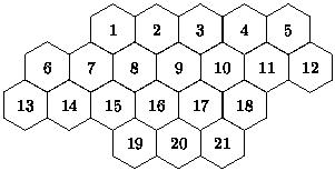
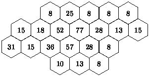
| Figure 1: Network structure Philadelpia instances | Figure 2: Demand of instance P1 |
The original instance and certain variants are widely used afterwards to substantiate algorithms and lower bounds for the MS-FAP. The Philadelphia instances are characterized by 21 hexagons denoting the cells of a cellular phone network around Philadelphia (see Figure 1). Until recently, it was common practice to model wireless phone networks as hexagonal cell systems. For each cell, a demand cv is given. Figure 2 shows the demand for the original instance P1, whereas the table below contains the demand vectors of all instances. In conformity with [Valenzuela et al., 1998], the instances are denoted by P1-P9. Some of them are also appointed in [Hurley et al., 1997] as E3-E9. In [Avenali et al., 2002] more variants are considered. These are numbered P1-P19. Since these names do not correspond with the ones in [Valenzuela et al., 1998] we rename them as p1-p19 (not all are included in this overview).
 |
 |
| Figure 3: Resuse distances P1, P3, P5, P7, P9 | Figure 4: Resuse distances P2, P4, P6 |
| instance | demand vector cv | reuse distances |
| P1 (E3,p3) | (8,25,8,8,8,15,18,52,77,28,13,15,31,15,36,57,28,8,10,13,8) | |
| P2 (E4,p8) | (8,25,8,8,8,15,18,52,77,28,13,15,31,15,36,57,28,8,10,13,8) | |
| P3 (E5,p2) | (5,5,5,8,12,25,30,25,30,40,40,45,20,30,25,15,15,30,20,20,25) | |
| P4 (E6,p7) | (5,5,5,8,12,25,30,25,30,40,40,45,20,30,25,15,15,30,20,20,25) | |
| P5 (E7,p1) | (20,20,20,20,20,20,20,20,20,20,20,20,20,20,20,20,20,20,20,20,20) | |
| P6 (p6) | (20,20,20,20,20,20,20,20,20,20,20,20,20,20,20,20,20,20,20,20,20) | |
| P7 (E8,p4) | (16,50,16,16,16,30,36,104,154,56,26,30,62,30,72,114,56,16,20,26,16) | |
| P8 (p9) | (8,25,8,8,8,15,18,52,77,28,13,15,31,15,36,57,28,8,10,13,8) | |
| P9 (E9,p5) | (32,100,32,32,32,60,72,208,308,112,52,60,124,60,144,228,112,32,40,52,32) |
| instance | lower bounds | optimal value (range) | upper bounds | ||||||||||||||||||
| [Gamst, 1986] | [Janssen and Kilakos, 1996a, Janssen and Kilakos, 1996b] | [Hurley et al., 1997, Smith et al., 1998] | [Sung and Wong, 1997] | [Heller, 2000] | [Avenali et al., 2002] | [Hurley et al., 1997] | [Hurley et al., 1997] | [Hurley et al., 1997] | [Valenzuela et al., 1998] | [Hurley et al., 1997, Smith et al., 1998] | [Allen et al., 1999] | [Smith et al., 2000a, Smith et al., 2000b] | [Beckmann and Killat, 1999b, Beckmann and Killat, 1999c] | [Matsui and Tokoro, 2001] | [Avenali et al., 2002] | [Sivarajan et al., 1989] | [Sung and Wong, 1997] | [Sung and Wong, 1997] | [Wang and Rushforth, 1996] | ||
| Graph Theory | Travelling Salesman Problem | Diverse methods | Graph Theory | Graph Theory | Integer Programming | Best Sequential Algorithm | Tabu Search | Simulated Annealing | Genetic Algorithm | Subgraph Extension | Subgraph Extension | Subgraph Extension | Genetic Algorithm | Genetic Algorithm | Integer Programming | Sequential Coloring | Generalized Sequential Packing 1 | Generalized Sequential Packing 2 | Local Search | ||
| P1 | 413 | 426 | 426 | 426 | - | 426 | 426 | 447 | 428 | 428 | 426 | 426 | - | - | - | 426 | 426 | 459 | 440 | 450 | 432 |
| P2 | 413 | 426 | 426 | 426 | - | 426 | 426 | 475 | 429 | 438 | 426 | 426 | - | - | 426 | 426 | 426 | 446 | 436 | 444 | - |
| P3 | 245 | - | 257 | 252 | - | 257 | 257 | 284 | 269 | 260 | 258 | 257 | - | - | - | 257 | 275 | 282 | 291 | 273 | 263 |
| P4 | 245 | 252 | 252 | 252 | - | 252 | 252 | 268 | 257 | 259 | 253 | 252 | - | - | 252 | 252 | 253 | 268 | 273 | 268 | - |
| P5 | 239 | - | 239 | 177 | - | 239 | 239 | 250 | 240 | 239 | 239 | - | - | - | - | 239 | 239 | - | - | - | - |
| P6 | 139 | 177 | 178 | 177 | 179 | 177 | 179 | 230 | 188 | 200 | 198 | - | 179 | - | - | 179 | 183 | - | - | - | - |
| P7 | 830 | - | 855 | 855 | - | 855 | 855 | 894 | 858 | 858 | 856 | 855 | - | - | - | 855 | 855 | - | - | - | - |
| P8 | 449 | - | 524 | 427 | - | 523 | 524 | 592 | 535 | 546 | 527 | - | - | 524 | - | 524 | 524 | - | - | - | - |
| P9 | 1,664 | - | 1,713 | 1,713 | - | 1713 | 1,713 | 1,800 | 1,724 | 1,724 | - | 1,713 | - | - | - | - | 1713 | - | - | - | - |
 zib.de